
Cluster Analysis
Intended Learning Outcomes
At the end of the cluster analysis sections students should be able to complete the following tasks.
- Define the following terms: divisive; agglomeratiave, monthetic, polythetic, distance.
- Explain the difference between a hierarchical and a non-hierarchical classification.
- Choose an appropriate distance measure.
- Decide if data should be standardised before measuring distance.
- Explain the differences between cluster algorithms beased on averages, distances, similarity and variance.
- Intrepret the relationships between cases from a dendrogram.
- Judge the quality of a classification.
- Select alternative clustering solutions that are likely to improve the usefulness of an analysis.
What is it?
Arranging objects into groups is a natural and necessary skill that we all share.
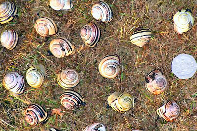
This ability is essential for biologists if we are to make sense out of the tremendous diversity of organisms, molecules, diseases, etc., that we are faced with. For example, the Cepea individuals collected from a Suffolk heathland (below) or the enormous amount of data derived from a microarray. As we shall see there are many possible rules that can be use to assign objects to groups, i.e. to classify them. For example, assigning a species name to a particular organism means that we are able to recognise it as belonging to a particular group.
The correct classification of organisms is so important that the biological discipline of taxonomy has been developed to deal with the theory and practice of biological classification.
Cluster analysis (CA) is a rather loose collection of statistical methods that is used to assign cases to groups (clusters). Group members share certain properties in common and it is hoped that the resultant classification will provide some insight into a research topic. The classification has the effect of reducing the dimensionality of a data table by reducing the number of rows (cases).
Try placing the following faces into groups. What criteria did you apply: size, hat, glasses, gender, hair colour? Is there a different classification that makes as much sense?
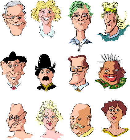
The above faces are the cases in their 'raw' state, i.e. before measurements and attributes have been recorded. More generally the starting point will be data that are already in a coded or numeric format. For example:
| case | sex | glasses | moustache | smile | hat |
|---|---|---|---|---|---|
| 1 | m | y | n | y | n |
| 2 | f | n | n | y | n |
| 3 | m | y | n | n | n |
| 4 | m | n | n | n | n |
| 5 | m | n | n | y? | n |
| 6 | m | n | y | n | y |
| 7 | m | y | n | y | n |
| 8 | m | n | n | y | n |
| 9 | m | y | y | y | n |
| 10 | f | n | n | n | n |
| 11 | m | n | y | n | n |
| 12 | f | n | n | n | n |
In these circumstances it may be less easy to see an obvious way of clustering the cases. Cluster analysis provides the tools that can cluster these cases in an objective manner.
Description and examples
The underlying mathematics of most of these methods is relatively simple but a large number of calculations is needed, which can make it impossible to undertake by hand and may even put a heavy demand on the computer.
The classification produced is very dependent upon the particular method used. This is because it is possible to measure similarity and dissimilarity in a number of ways. Consequently there is no such thing as a single correct classification, although there have been attempts to define concepts such as 'optimal' classifications.
Some Terminology
As with all statistical methods there is some important terminology that must be mastered. Before continuing to the next section ensure that you fully understand all of the terms described below.
hierarchical
Most CA techniques are hierarchical, i.e, the resultant classification has an increasing number of nested classes. The result resembles a phylogenetic classification. Others are non-hierarchical methods, for example k-means clustering.
divisive or agglomerative
Clustering techniques can be divisiveor agglomerative.A divisive method begins with all cases in one cluster. This cluster is gradually broken down into smaller and smaller clusters. Agglomerative techniques start with (usually) single member clusters. These are gradually fused until one large cluster is formed.
monothetic or polythetic
In a monothetic scheme cluster membership is based on the presence or absence of a single characteristic. Polythetic schemes use more than one characteristic (variables). For example, classifiying people solely on the basis of their gender is a monthetic classification, but if both gender and handedness (left, right handed) are used the classification is polythetic.
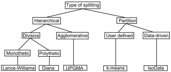
The following diagram is based on Figure 6 in Grabmeier and Rudolph (2002). It is a taxonomy of clustering algorithms and the final box (bottom row) is one representative algorithm. Note that other methods could have been chosen as representatives
These notes concern polythetic agglomerative methods. Work your way through the next three sections before attempting the self assessment exercises. You may find it helpful to make notes as you progress.
Summary of a polthethetic, agglomerative classification
The complete process of generalised hierarchical clustering can be summarised as follows:
- Decide which data to record from your cases. You may need to think carefully about datatypes since it is very difficult to mix data types in a cluster analysis. For example, interval data such as weight cannot be easilly combined with attirbute data such as blood group.
- Calculate the distance between all initial clusters. Store the results in a distance matrix. In most analyses initial clusters will be made up of individual cases, thus at the start the number of clusters will equal the number of cases.
- Search through the distance matrix and find the two most similar clusters. If several pairs share the same similarity use a pre-determined rule to decide between the alternatives.
- Fuse these two clusters to produce a cluster that now has at least 2 cases. The number of clusters decreases by one.
- Calculate the distances between this new cluster and all other clusters (which may contain only one case). There is no need to recalculate all the distances since only those involving the new cluster will have changed.
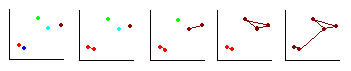
- Repeat step 3 until all cases are in one cluster. The process described above is summarised in the diagram below. The red and blue cases are the closest together so are fused to form a cluster (red). Next the brown and blue cases are fused to form a cluster (brown). The green case is fused with the brown cluster. At this stage there are two clusters and there is no alternative but to fuse these two.
The diversity of clustering methods arises because there are many ways of measuring distances and many different places between which distances can be measured. These aspects are covered in A and B in the next section.
1 |
Appropriate classificationsImagine that you have presented a shuffled deck of cards to a colleague and asked them turn over the cards one by one and place them into groups (clusters). Which of the following groups would be appropriate? Note that more than one could be appropriate. |
Analysis steps
Undertaking a cluster analysis involves a series of decisions that have a profound effect on the outcome. The list below takes you through the steps and then details some example analyses. There are are also links to the datafiles and self-assessment exercises.
A. Measuring the similarity between objects
B. Joining groups together
C. The dendrogram
D. Examples
E. Cluster
Analysis using Minitab
F. Self assessment exercises
Resources
Books
- Everitt, B. S., Landau, S. and Leese, M. 2001. Cluster Analysis, 4th edition. Edward Arnold.
- Gordon, A. D. 1980 and 1990. Classification.Chapman and Hall.
- Jongman, R. H. G., ter Braak, C. J. F. and van Tongeren, O. F. R. 1995. Data analysis in community and landscape ecology. Cambridge University Press.
- Kaufmann, L. and Rousseeuw, P. J. 1990. Finding groups in data: an introduction to cluster analysis. Wiley.
- Legendre, P. and Legendre, L. 1998. Numerical Ecology (2nd English edition). Elservier, Amsterdam.
- Sneath, P. H. A. and Sokal, R. R. 1973. Numerical Taxonomy. Freeman & Co.
- Stuetzle, W. 1995. Data Visualization and Interactive Cluster Analysis. ICPSR, Ann Arbor, MI.
Internet resources
- Statsoft's cluster analysis explanations
- Cluster and TreeView are an integrated pair of programs for analyzing and visualizing the results of complex microarray experiments. Both written by Michael Eisen.
- Pierre Legendre's k-means clustering program is available in Mac and Windows versions.
- Bioinformatics Software: AMIADA (Analyzing Microarray Data), Mac & Windows versions.
Printed and Electronic papers
- Chipman, H. and Tibshirani, R. 2005. Hybrid Hierarchical Clustering with Applications to Microarray Data. Biostatistics, online publication doi:10.1093/biostatistics/kxj007. Available in pdf format from http://www-stat.stanford.edu/~tibs/ftp/chipman-tibshirani-2003-modified.pdf.
- Eisen, M. B., Spellman, P. T., Browndagger, P. O. and Botstein, D. 1998. Cluster analysis and display of genome-wide expression patterns. Proceedings National Academy of Science, USA, 95(25): 14863-14868. Available electronically from http://www.pnas.org/cgi/reprint/95/25/14863.
- Golub, T. R. Slonim, D. K. Tamayo, P., Huard, C., Gaasenbeek, M., Mesirov, J. P., Coller, H., Loh, M., Downing, J. R., Caligiuri, M. A., Bloomfield, C.D. and Lander, E. S. 1991. Molecular Classification of Cancer: Class Discovery and Class Prediction by Gene Expression. Science, 286: 531-536. (available as a pdf file, plus associated data files from http://www.broad.mit.edu/cgi-bin/cancer/publications/pub_paper.cgi?mode=view&paper_id=43) .
- Hastie, T., Tibshirani, R. Eisen, M. B., Alizadeh, A., Levy, R., Staudt, L., Chan, W. C., Botstein, D. Brown, P. 2000. 'Gene shaving' as a method for identifying distinct sets of genes with similar expression patterns. Genome Biology, 1(2): research0003.1-0003.21. The electronic version is available online at http://genomebiology.com/2000/1/2/research/0003.
- Lapointe, F. J. and Legendre, P. 1994. A Classification of Pure Malt Scotch Whiskies. Applied Statistics, 43(1): 237-25. Also available electronically in a modified form from http://www.dcs.ed.ac.uk/home/jhb/whisky/lapointe/text.html
- Pillar, V. D. 1999. How sharp are classifications? Ecology, 80: 2508-2516.
- Proches, S. 2005. The world's biogeographic regions: cluster analysis based on bat distributions. Journal of Biogeography, 32: 607-614.
- Riordan, P. 1998. Unsupervised recognition of individual tigers and snow leopards from their footprints. Animal Conservation, 1: 253-262.
- Schmelzer, I. 2000. Seals and seascapes: covariation in Hawaiian monk seal subpopulations and the oceanic landscape of the Hawaiian Archipelago. Journal of Biogeography, 27:901-914.
- Tibshirani, R., Hastie, T. Eisen, M., Ross, D. , Botstein, D. and Brown, P. 1999. Clustering methods for the analysis of DNA microarray data. Technical report, Department of Statistics, Stanford University. Available for download as a postscript file from http://www-stat.stanford.edu/~tibs/ftp/sjcgs.ps