k-means procedure
This method differs from hierarchical clustering in many ways. In particular:
- There is no hierarchy, the data are partitioned. You will be presented only with the final cluster membership for each case.
- There is no role for the dendrogram in k-means clustering.
- You must supply the number of clusters (k) into which the data are to be grouped.
At the end of the analysis the data are split between k clusters (where you decide what value to assign to k).
The method is conceptually simple but computationally intensive. At its simplest:
- Cases are initially assigned randomly to the k clusters. Imagine that you split a shuffled deck of cards into two parts (k = 2).
- Cases are then moved around between clusters using an iterative method so that a classification is produced such that the clusters must be internally similar, but externally dissimilar to other clusters.
- The analysis stops when moving any more cases between clusters would makes the clusters become more variable. For example, in the card example we might end up with a set of red cards and a set of black cards.
Cluster variability is measured with respect to their means for the classifying variables, hence the name k-means clustering. If more than one variable is used to define the clusters the distances (dissimilarities) between clusters are measured in multi-dimensional space (e.g. euclidean distance).
K-means using Minitab
The following example describes how to undertake a k-means clustering using Minitab. The data analysed are the February weather conditions in Bradford.
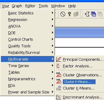
K-means clustering is obtained from the multivariate sub-menu from the stats menu.

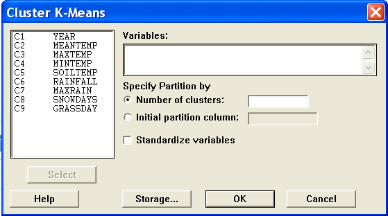
The opening screen is quite simple and asks for
- the variables to use for the clustering;
- the number of clusters (k)
- and whether data standardisation is required.

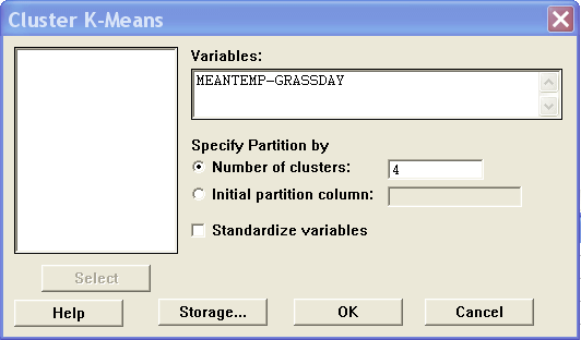
There is also an option to store the cluster membership. In this analysis all of the varaibles, except year, are used in a standardised format with k equal to 4. Cluster membership is strored in an additional column.

K-means cluster results
Cluster membership for each year is shown below. 1986 stands out as an unusual year
  1 1982
  1 1992
  1 1993
  2 1986
  3 1984
  3 1987
  3 1988
  3 1989
  3 1990
  3 1991
  4 1983
  4 1985
Details of the analysis are given below. [skip]
Standardized Variables
Final Partition
Number of clusters: 4
        Number of     Within cluster  Average distance  Maximum distance
        observations  sum of squares  from centroid     from centroid
  Cluster1   3           1.949           0.806             0.825
  Cluster2   1           0.000           0.000             0.000
  Cluster3   6          29.074           2.008             3.449
  Cluster4   2           1.565           0.885             0.885
The above table shows that cluster 3 has the most variability.
Cluster Centroids [[skip table]]

  Variable Cluster1 Cluster2 Cluster3 Cluster4 Grand centrd

  MEANTEMP  0.6320  -1.9693  0.3160  -0.9112   0.0000
  MAXTEMP   0.2861  -2.6300  0.5449  -0.7489  -0.0000
  MINTEMP   0.3650  -1.7550  0.2246  -0.3440   0.0000
  SOILTEMP  0.7125  -1.7575  0.1289  -0.5768   0.0000
  RAINFALL -0.6989  -0.8488  0.7870  -0.8885  -0.0000
  MAXRAIN  -0.7554  -1.0072  0.8183  -0.8183   0.0000
  SNOWDAYS -0.5779   2.5949 -0.2153   0.2153  -0.0000
  GRASSDAY -0.7804   1.4828 -0.0780   0.6634  -0.0000
The above table gives the means (standardised) for each cluster. Recall that negative values indicate below average values, positive values are above average. This means that cluster 1 is above average for the temperature variables and below average for the other variables (warm, dry years?). Cluster 3 is also above average on the temperature variables, but also on the rainfall variables (warm and wet years?). Cluster 4 years appear to have been colder, with below average rainfall but aove average snowfall. Cluster 2 (1986) seems to have been very different from all other years in being particularly cold and snowy (I remember it well!). [[skip table]]
	Distances Between Cluster Centroids

            Cluster1  Cluster2  Cluster3 Cluster4
  Cluster1  0.0000    6.4141    2.4159   2.8933
  Cluster2  6.4141    0.0000    6.2548   3.7966
  Cluster3  2.4159    6.2548    0.0000   3.1973
  Cluster4  2.8933    3.7966    3.1973   0.0000
Return to Cluster Analysis
