
The Dendrogram
Background
Understanding how a dendrogram is constructed, and how it should be interpreted, is one of the most important aspects of cluster analysis. It will be demonstrated by a simple example that ignores a lot of 'messy' details. The calculations, and resultant dendrogram, would change with a different distance measure and/or clustering algorithm.
Sample data
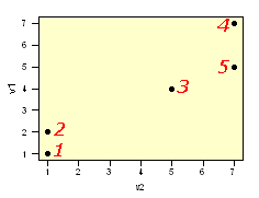
The data set has 5 cases and two variables (v1 & v2)
| case | v1 | v2 |
|---|---|---|
| 1 | 1 | 1 |
| 2 | 2 | 1 |
| 3 | 4 | 5 |
| 4 | 7 | 7 |
| 5 | 5 | 7 |
These data are used to calculate a euclidean distance matrix. Note that only the lower triangle is given since the distance between cases 2 & 4 is the same as that between cases 4 & 2. Distances are presented with 2 significant figures.
Details
| 1 | 2 | 3 | 4 | 5 | |
|---|---|---|---|---|---|
| 1 | 0.0 | ||||
| 2 | 1.0 | 0.0 | |||
| 3 | 5.0 | 4.5 | 0.0 | ||
| 4 | 8.5 | 7.8 | 3.6 | 0.0 | |
| 5 | 7.2 | 6.7 | 2.2 | 2.0 | 0.0 |
Using these distances the most similar pair of cases is 1 and 2.
| 1 | 2 | 3 | 4 | 5 | |
|---|---|---|---|---|---|
| 1 | 0.0 | ||||
| 2 | 1.0 | 0.0 | |||
| 3 | 5.0 | 4.5 | 0.0 | ||
| 4 | 8.5 | 7.8 | 3.6 | 0.0 | |
| 5 | 7.2 | 6.7 | 2.2 | 2.0 | 0.0 |
These two cases are fused to form the first cluster. Distances must now be calculated between this cluster and the other 3 cases. For the purpose of this exercise assume that distances are calculated from the means of v1 and v2, i.e. mean v1 = 1.5, mean v2 = 1.0. This produces a revised distance matrix (cases 1 & 2 have been removed and replaced by A, the first cluster).
| A | 3 | 4 | 5 | |
|---|---|---|---|---|
| A | 0.0 | |||
| 3 | 4.7 | 0.0 | ||
| 4 | 8.1 | 3.6 | 0.0 | |
| 5 | 6.9 | 2.2 | 2.0 | 0.0 |
The smallest distance in this matrix is between cases 4 & 5 (distance = 2.0). These will be fused to form cluster B (means: v1 = 6, v2 = 7). These new values are used to recalculate the distance matrix.
| A | B | 3 | |
|---|---|---|---|
| A | 0.0 | ||
| B | 7.5 | 0.0 | |
| 3 | 4.7 | 2.8 | 0.0 |
The new smallest distance is between cluster B and case 3: 2.8. Thus case 3 is fused with cluster B and cluster B now has 3 members. The mean values are: v1 = (4+5+7)/3 = 5.3, v2 = (5+7+7)/3 = 6.3). Obviously, there are now only 2 clusters and they must be the next to be fused, distance = 6.4.
| A | B | |
|---|---|---|
| A | 0.0 | |
| B | 6.4 | 0.0 |
The Dendrogram
The entire process of fusions is now summarised by the dendrogram.
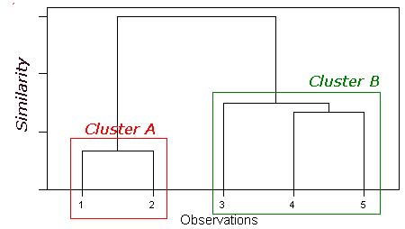
It appears, from this dendrogram, that the data can be represented by 2 clusters (A & B). However, as the number of cases increases it may not be so obvious. Indeed, one of the biggest problems with this Cluster Analysis is identifying the optimum number of clusters. As the fusion process continues increasingly dissimilar clusters must be fused, i.e. the classification becomes increasingly artificial. Deciding upon the optimum number of clusters is largely subjective, although looking at a graph of the level of similarity at fusion versus number of clusters may help. There will be sudden jumps in the level of similarity as dissimilar groups are fused.
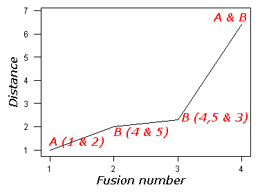
The following plot is derived from our sample data. Note how there is a large jump when clusters A & B are fused. This supports the hypothesis that the data are best represented by two clusters.
Return to Cluster Analysis.