Principal Components Analysis
Principal Components Analysis with rotation
The first analysis is a 'pure' PCA using all variables, except for Region. Factor scores have been saved and all graph options selected.
Eigenanalysis of the Correlation Matrix
Eigenvalue |
4.6505 |
2.1944 |
1.2284 |
1.1201 |
0.915 |
0.7011 |
|---|---|---|---|---|---|---|
Proportion |
0.3880 |
0.1830 |
0.1020 |
0.0930 |
0.076 |
0.0580 |
Cumulative |
0.3880 |
0.5700 |
0.6730 |
0.7660 |
0.842 |
0.9010 |
Eigenvalue |
0.4477 |
0.308 |
0.210 |
0.1365 |
0.0514 |
0.0369 |
|---|---|---|---|---|---|---|
Proportion |
0.0370 |
0.026 |
0.017 |
0.0110 |
0.0040 |
0.0030 |
Cumulative |
0.9380 |
0.964 |
0.981 |
0.9930 |
0.9970 |
1.0000 |
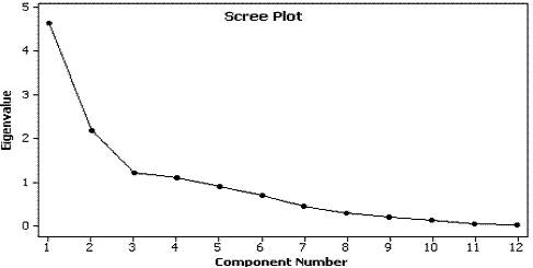
Scree plot
 [D]
[D]
1 |
Effective dimensionality from the eigen values.Which of the following statements is a reasonable description of the effective dimensionality of these data? |
Variable |
PC1 |
PC2 |
PC3 |
PC4 |
PC5 |
PC6 |
|---|---|---|---|---|---|---|
MaxAlt |
0.407 |
0.053 |
-0.176 |
-0.351 |
-0.109 |
-0.013 |
MeanAlt |
0.357 |
-0.110 |
0.023 |
-0.472 |
-0.151 |
0.031 |
SDAlt |
0.384 |
0.186 |
-0.320 |
-0.091 |
0.042 |
-0.024 |
MeanSlope |
0.357 |
0.196 |
-0.336 |
-0.040 |
0.267 |
-0.083 |
Mire |
-0.235 |
-0.154 |
0.138 |
-0.563 |
-0.258 |
0.473 |
Heathland |
0.326 |
-0.079 |
0.086 |
0.333 |
-0.035 |
0.302 |
WetHeath |
-0.106 |
0.311 |
-0.115 |
0.026 |
-0.777 |
-0.446 |
Deer |
0.326 |
0.070 |
0.225 |
0.248 |
-0.331 |
0.444 |
Sheep |
-0.214 |
-0.366 |
-0.522 |
-0.152 |
0.053 |
0.038 |
Cattle |
0.099 |
-0.617 |
-0.094 |
0.109 |
-0.124 |
-0.241 |
NPP |
-0.196 |
0.096 |
-0.618 |
0.271 |
-0.208 |
0.458 |
Grazed |
0.242 |
-0.507 |
0.008 |
0.213 |
-0.223 |
-0.100 |
Variable |
PC7 |
PC8 |
PC9 |
PC10 |
PC11 |
PC12 |
|---|---|---|---|---|---|---|
MaxAlt |
0.056 |
-0.105 |
-0.121 |
0.200 |
0.038 |
-0.771 |
MeanAlt |
0.136 |
-0.460 |
-0.316 |
-0.225 |
-0.108 |
0.470 |
SDAlt |
-0.069 |
0.334 |
0.120 |
0.632 |
-0.007 |
0.419 |
MeanSlope |
-0.058 |
0.335 |
0.211 |
-0.694 |
0.008 |
-0.002 |
Mire |
-0.219 |
0.485 |
0.063 |
-0.083 |
0.036 |
0.006 |
Heathland |
-0.788 |
-0.156 |
-0.171 |
-0.027 |
-0.011 |
-0.021 |
WetHeath |
-0.230 |
-0.004 |
0.091 |
-0.113 |
0.013 |
0.038 |
Deer |
0.347 |
-0.117 |
0.563 |
-0.032 |
-0.134 |
-0.011 |
Sheep |
-0.195 |
-0.420 |
0.523 |
0.038 |
0.177 |
0.021 |
Cattle |
0.017 |
0.232 |
0.002 |
0.000 |
-0.676 |
-0.061 |
NPP |
0.231 |
0.025 |
-0.419 |
-0.061 |
-0.098 |
0.001 |
Grazed |
0.189 |
0.223 |
-0.137 |
-0.051 |
0.685 |
0.052 |
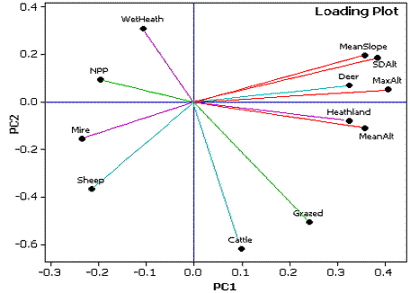
Loading plot (modified from Minitab default)
 [D]
[D]
2 |
CoefficientsMatch the coefficient to the variable / component (PC1 to PC6 only). |
3 |
Interpreting the coefficientsWhich of the following statements can be justified? |