
Outline of eigen analysis methods
2 x 2 matrices
- The calculation of eigenvalues (also known as latent roots) and eigen vectors is a unique matrix algebra operation that plays a very important role in many of the multivariate methods.
- It is also known as 'Single Value Decomposition'.
- It provides a summary of the data structure represented by a symmetrical matrix (such as would be obtained from correlations, covariances or distances).
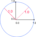
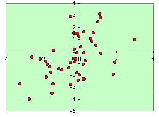
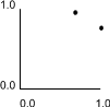
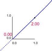
Understanding of the underlying principles is essential for many multivariate methods. The relevance of these values is shown graphically. (See the book, Statistics and Data Analysis for Geologists by Davis for a more complete description of this and matrix methods in general). This demonstration is of an eigen alysis restricted to a simple 2 x 2 matrix. This restriction facilitates a graphical description.Consider the following matrix in which the rows are the coordinates of a pair of points in 2-D space.
4 8
8 4
Graphically these points would be positioned as shown below.
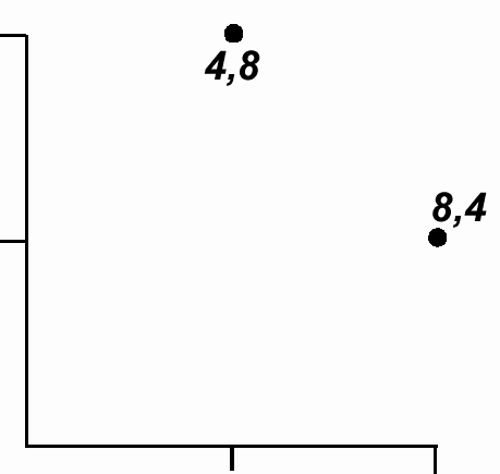
Using the 0,0 coordinate as its centre it is possible to construct an ellipse, such that the two points fall on its perimeter.
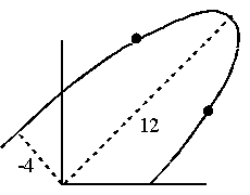
- A 2 x 2 matrix has two eigenvalues.
- In the above example they are 12 and -4, which are the lengths of the major and minor axes of the ellipse that encloses the points.
- Eigen values can only be found for a square symmetric matrix (all correlation and covariance matrices are symmetrical, as are most distance matrices) and there will be as many eigen values as there are rows in the matrix.
- There is an eigenvector associated with each of eigenvalue.
Eigenvectors
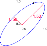
If you wish to draw the axes of the ellipse you need, in addition to their lengths, information about their direction. Eigen vectors are the coordinates that define the direction of the axes, whose lengths are given by the eigen values. However, eigenvectors, which are centered at 0,0, do not have unique values, each has an infinite number of possible values. This is because any coordinate on an axis allows it to be drawn.
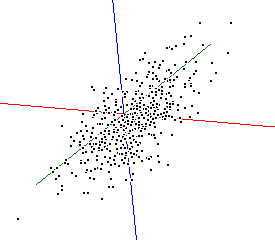
Correlations and eigenvalues
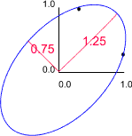
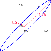
Although not justified here, it is possible to represent correlations as vectors. Again, for simplicity, the explanation is first restricted to two dimensions. In the following plots two variables are shown, that become increasingly correlated. The format of the correlation matrices is:
| correlation of x with x | correlation of x with y |
| correlation of y with x | correlation of y with y |
Note that a variable correlated with itself always has a correlation coefficient of 1.00, and that the correlation of x with y is the same as that for y with x. Hence the matrices are symmetrical. The rows in these matrices form the coordinates for two points. Also shown on the plots are the major and minor axes of the enclosing ellipses. The lengths of these axes are the eigenvalues of the correlation matrices. Thus, for the first matrix they are 1 & 1, for the second 1.25 & 0.75, etc. Note that the eigen values sum to 2, which is the number of variables.
| 1.00 | 0.00 |
| 0.00 | 1.00 |
 |
 |
 |
| 1.00 | 0.25 |
| 0.25 | 1.00 |
 |
 |
 |
| 1.00 | 0.50 |
| 0.50 | 1.00 |
 |
 |
 |
| 1.00 | 0.75 |
| 0.75 | 1.00 |
 |
 |
 |
| 1.00 | 1.00 |
| 1.00 | 1.00 |
 |
 |
 |
An obvious question but, what trends do you notice in the above plots?
As the variables become more correlated the major axis becomes longer whilst the minor axis becomes proportionately shorter. The limit is reached when the two variables are perfectly correlated. Under these conditions the major axis has a length of 2.0, whilst the minor axis has a length of 0.
- The eigen vectors for the first axes share the same values.
- This is because they share the same direction.
- The eigen vectors have the values of 0.707 (on the x axis) and 0.707 (on the y axis).
- Why these two values when any pair of coordinates, such as 0.5 & 0.5, would also be applicable?
- The chosen coordinates share a special relationship such that the sum of their squared values equals 1, i.e.
0.7072 + 0.7072 = 0.4998 + 0.4998 = 1.00 (within the limits of the significant figures employed).
This is a commonly applied scaling for eigen vectors, it is certainly used in many multivariate statistical packages.
Note that the eigen vectors for the minor axis also share the same coordinates: 0.707 and -0.707. The equality of these eigen vectors is an artefact imposed by the two dimensional limit.
Extending beyond two dimensions
Similar relationships apply for any symmetrical matrix. For example, in a 3 x 3 matrix each point is now defined by x, y & z values. An ellipsoid could be drawn around these data (think of the ellipsoid as a rugby football). There would now be three eigen values, and their associated eigenvectors, which correspond to the three axes of the ellipsoid.
 |
 |
Consider the following 3 by 3 scatter plots and their associated correlation matrices. Only the lower triangles are shown.
Scatter plot 1
| x | y | z | Eigenvalues | vector 1 | vector 2 | vector 3 | ||
|---|---|---|---|---|---|---|---|---|
| x | 1.0 | 1.0 | 0.000 | 0.000 | 1.000 | |||
| y | 0.0 | 1.0 | 1.0 | 0.000 | 1.000 | 0.000 | ||
| z | 0.0 | 0.0 | 1.0 | 1.0 | 1.000 | 0.000 | 0.000 |
Scatter plot 2
| x | y | z | Eigenvalues | vector 1 | vector 2 | vector 3 | ||
|---|---|---|---|---|---|---|---|---|
| 1.0 | 2.0 | -0.577 | 0.085 | -0.812 | ||||
| 0.5 | 1.0 | 0.5 | -0.577 | -0.746 | 0.332 | |||
| 0.5 | 0.5 | 1.0 | 0.5 | -0.577 | 0.660 | 0.480 |
Scatter plot 3
| x | y | z | Eigenvalues | vector 1 | vector 2 | vector 3 | ||
|---|---|---|---|---|---|---|---|---|
| 1.0 | 3.0 | -0.577 | 0.000 | 0.000 | ||||
| 1.0 | 1.0 | 0.0 | -0.577 | 0.000 | 0.000 | |||
| 1.0 | 1.0 | 1.0 | 0.0 | -0.577 | 0.000 | 0.000 |
Scatter plot 4
| x | y | z | Eigenvalues | vector 1 | vector 2 | vector 3 | ||
|---|---|---|---|---|---|---|---|---|
| 1.0 | 2.23 | 0.593 | -0.525 | 0.611 | ||||
| 0.9 | 1.0 | 0.73 | 0.658 | -0.121 | -0.743 | |||
| 0.3 | 0.6 | 1.0 | 0.04 | 0.464 | 0.842 | 0.273 |
Again, note how the correlation structure affects the eigen values. As the variables become more correlated so the length of the first eigen value increases. Note also that the sum of the squared eigen vectors equals 1.0, e.g -0.5772 + -0.5772 + -0.5772 = 1.00.
Try to guess the approximate sizes of the eigen values for the next three 4 by 4 correlation matrices (variables are labelled a, b c and d). Recall that the sum of the eigen values will be 4.0. You are not expected to guess an exact value, rather the relative magnitudes.
| 1 |
a
|
b
|
c
|
d
|
|
|---|---|---|---|---|---|
| a | 1.00 | ||||
| b | 0.00 | 1.00 | |||
| c | 0.00 | 0.00 | 1.00 | ||
| d | 0.00 | 0.00 | 0.00 | 1.00 | |
| 2 | a | b | c | d | |
| a | 1.00 | ||||
| b | 0.90 | 1.00 | |||
| c | 0.00 | 0.00 | 1.00 | ||
| d | 0.00 | 0.00 | 0.90 | 1.00 | |
| 3 | a | b | c | b | |
| a | 1.00 | ||||
| b | 0.90 | 1.00 | |||
| c | 0.20 | 0.30 | 1.00 | ||
| d | 0.15 | 0.10 | 0.80 | 1.00 |
The answers are:
- 1.00, 1.00, 1.00, 1.00
- 1.90, 1.90, 0.10, 0.10
- 2.23, 1.48, 0.23, 0.06
|
1 |
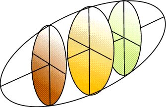
Self-Assessment Question: Data structure of correlation matricesDecide which of the listed objects is a reasonable approximation to the shape of the data summarised by the following correlation matrices. Matrix M1 Matrix M2 Matrix M3 Matrix M4 |
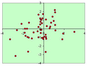
Why is eigen analysis so useful?
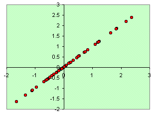
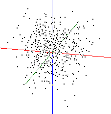
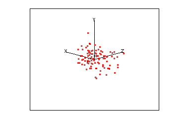
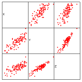
Imagine a set of data in 3-D space, i.e. where each point is defined by a x,y & z coordinate. Assume that these points are arranged in a cloud of points which resemble a rugby football.
| An animated 3-D plot | Matrix of equivalent 2 x 2 plots |
|---|---|
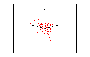 |
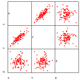 |
As this cloud of points rotates you should notice that it is very flat in one plane, this should be reflected in one small eigen value. The correlation for these three variables is:
| x | y | z | |
|---|---|---|---|
| x | 1.00 | ||
| y | 0.86 | 1.00 | |
| z | 0.02 | 0.06 | 1.00 |
giving three eigen values of 1.865, 1.003 and 0.132. Re-examine the animated plot and the 2-D matrix plots now that you know the eigenvalues of the correlation matrix. Can you understand how these eigen values relate to this set of multivariate data?
- The major axis of these points passes along the direction of greatest variability, i.e. the biggest range of values.
- The second axis identifies the second greatest direction of variability, which is uncorrelated (orthogonal) with the first, and so on.
- The third eigen value is small because the ellipsoid is thin (shaped a little like a pitta bread).
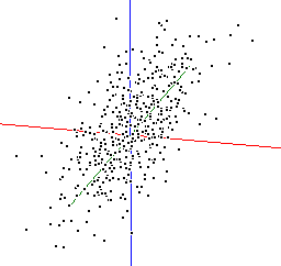
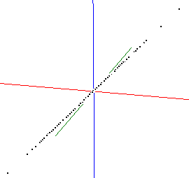
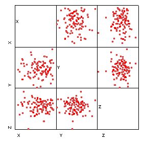
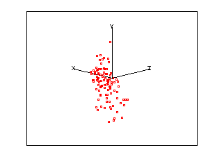
Two more examples are presented below.
| Example 1 | |||||||||||||||||
|
|
||||||||||||||||
 |
 |
||||||||||||||||
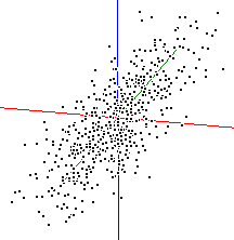
| Example 2 | |||||||||||||||||
|
|
||||||||||||||||
 |
 |
These axes are defined by the eigenvalues and eigen vectors of a matrix derived from the original data. They provide information about the dimensionality of the data and how the variables are related to each other and the main axes through the 'data cloud'.
Another way of understanding these new axes is to consider that when an ellipsoid's axes are drawn they are, in effect, new variables derived from the existing ones. This is a different approach to understanding multivariate data that froms the basis of PCA. It is, however, important to remember that it is the eigen analysis methods that provide a method for defining these new variables.
A simple way of creating a new variable is to make it a sum, i.e. a linear combination, of existing variables. This is explored in the next section.