Decision trees in more detail
Evaluating splits
In the simple example it was easy to see where the best split should be placed. It is less simple with real data and an algorithm is needed that evaluates possible splits. Several algorithms have been used but they share a common aim of favouring homogeneous nodes and heterogeneity between the child nodes. The homogeneity within a node is related to the "node impurity", with the aim being finding the splits that produce child nodes with minimum impurity.
A node is pure (impurity = 0) when all cases have the same value for the response or target variable, e.g. Node 2 above. A node is impure if cases have more than one value for the response, e.g. Node 1 above. The two most common methods for measuring node impurity are Gini and Entropy. It turns out that they produce similar results. If you wish to find out more about these measures see Chapter 5 of the book Machine Learning, Neural and Statistical Classification edited by Michie et al. CTREE uses an entropy calculation.
Assigning Categories to Nodes
Terminal nodes are assigned a response value or label, male or female in the above example. All cases in the node will be assigned this value. For example, all cases in Node 5 above will be labeled as males, even though one case is female. While it is reasonably clear in the artificial example how labels should be assigned it is less clear in real examples, particularly if unequal misclassification costs are applied. Labels are assigned to minimize the misclassification cost for the cases in the node. If misclassification costs are the same (the same cost to label a male as a female as it is to label a female as a male) the node label is the category with the most cases. The calculation of misclassification costs when costs are unequal are not covered here but can be found in Michie et al. CTREE does not allow unequal costs.
Dealing with missing predictor values
If a value is missing, for example someone refused to be weighed, it may be impossible to apply a rule to the case. Most decision tree programs deal with this problem by using a sophisticated technique involving surrogate variables. This method uses the values from non-missing variables to estimate the missing value. For example, in this artificial example height and weight have a high correlation coefficient of 0.75. Therefore, a reasonable estimate of a missing weight can be found from the height. The implementation of surrogate variables is quite sophisticated because it adjusts the identity of the surrogates depending on the node. CTREE uses a very simple missing value algorithm instead of surrogate variables.
Stopping Criteria
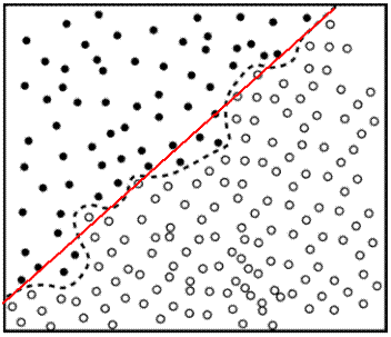
All decision trees need stopping criteria or it would be possible, and undesirable, to grow a tree in which each case occupied its own node. The resulting tree would be computationally expensive, difficult to interpret and would probably not work very well with new data. For example, consider the diagram below. The dotted curve is a decision boundary that accurately separates out the two classes in the training data. A diagonal red line is probably a better decision boundary for new cases.

The stopping criteria used by CTREE are typical of many decision tree programs.
- Number of cases in the node is less than some pre-specified limit.
- Purity of the node is more than some pre-specified limit. Because CTREE only allows equal costs this means that the proportion of cases in the node with class equal to the majority class is more than the pre-specified limit.
- Depth of the node is more than some pre-specified limit.
- Predictor values for all records are identical - in which no rule could be generated to split them.
Pruning Trees
A related problem is deciding on the optimum tree size. While stopping criteria are a relatively crude method of stopping tree growth, early studies showed that they tended to degrade the tree's performance. An alternative approach to stopping growth is to allow the tree to grow and then prune it back to an optimum size.
If tree performance is measured from the number of correctly classified cases it is common to find that the training data (a technique called re-substitution) gives an over-optimistic guide to future performance, i.e. with new data. Indeed if the tree was large enough it could be 100% accurate - unless two cases with different labels had identical values for all predictors. Ideally, all classifiers, such as decision trees, should exhibit generalization, i.e. work well with data other than those used to generate the tree. Although it may seem counter-intuitive as the tree grows it often shows a decrease in generalization. This is because the deeper nodes are fitting noise in the training data rather than the real signals that discriminate the classes. Therefore, pruning the tree back so that this 'over-fitting' is removed will improve generalisation.

One of the most common pruning methods used to improve generalization is k-fold cross validation. This makes use of the existing data to simulate independent test data.
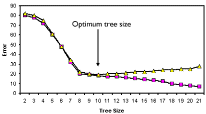
First, all of the data are used and the tree is allowed to grow as large as possible. This is the reference, unpruned tree. This will give the best performance with the training data - a tree size of 21 nodes in the above diagram.
The training data are next partitioned into k groups called "folds". Usually, an attempt is made to keep the same class frequencies in each fold. There is considerable research which shows that little is gained if k goes above 10. Each of the 10 folds will be used as an 'independent' test set while the other 9 form the training set. This means that there will be 10 separate training and test data sets - although the training sets will always share a large number of the same cases.
This means that 10 separate trees will generate an error rate for each of the 10 test data sets. These 10 error rates are averaged to produce an error rate as a function of tree size. This information can then be used to prune the reference tree to the number of nodes that produces the minimum error from the cross-validated trees. Pruning starts at the terminal nodes and proceeds in a stepwise fashion, sequentially removing the least important nodes until the desired size is reached. In the above example a tree with 10 nodes gives the lowest error with the test data.
The cross-validated trees are only used as a guide to the optimum tree size, the tree structure is of no interest.
The end product of this process is a pruned reference tree which should produce the optimum performance with new data.
CTREE prunes using a pessimistic error rate at the node. At the node a 50% confidence interval of the error rate is computed and its upper limit is taken as the pessimistic error rate. If the pessimistic error rate of a node is less than that of the subtree rooted at that node, the node is pruned.