Example Analysis 1
These analyses use the example file PCA_EG1.MTW (available from the Data Files link on the WebCT unit homepage). This is the data file used in the first of the example analyses.
PCA and Factor Analysis are available from the Minitab Stat menu via the Multivariate option.
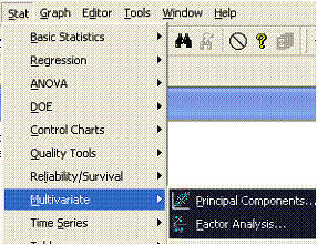
PCA
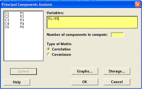
PCA Options
The important options are highlighted in yellow.
- You must select some variables to analyse
- Leave the Number of Components blank unless you have a reason to change the default.
- Leave Correlation as the type of matrix.
Graph Options
The graphs option offers three alternatives - see example analysis later.

Storage Options
The storage option allows you to save the PC coefficients and/or the component scores. Ensure that you specify as many columns as are required, otherwise you get an error message.

Example Minitab Output
This is the output from the above.
Principal Component Analysis: V1, V2, V3, V4, V5
Eigenanalysis of the Correlation Matrix
Eigenvalue    2.4480    1.6518    0.5110    0.3044    0.0848
Proportion     0.490     0.330     0.102     0.061     0.017
Cumulative     0.490     0.820     0.922     0.983     1.000
Variable         PC1       PC2       PC3       PC4       PC5
V1            -0.513     0.262     0.479     0.628    -0.208
V2            -0.605    -0.132    -0.229    -0.015     0.751
V3            -0.587    -0.077    -0.383    -0.358    -0.611
V4            -0.123    -0.651     0.666    -0.342    -0.017
V5             0.101    -0.695    -0.357     0.600    -0.138
If the above analysis is repeated but all three graph options are selected the output is identical to the above apart from the following graphs.
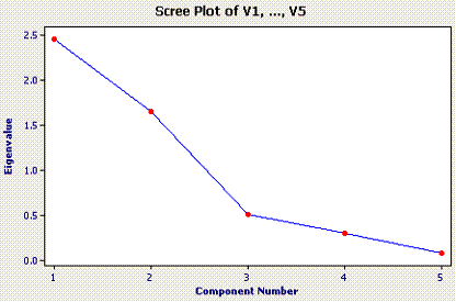
Scree plot
The scree plot (the eigen values plotted sequentially from first to last) suggests that 3 components should be used / extracted. This is because the slope is quite steeply downwards from PC1 to PC3, at which the slope is abruptly less.
Score Plot
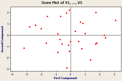
The score plot plots the component 1 scores against the component 2 scores. This a scatter plot of the values of the new components (PC1 and PC2) for each case. In this example the points are spread evenly between the four quadrants.
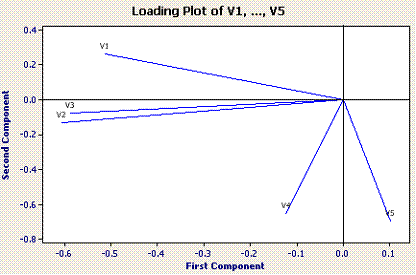
Loading Plot
This is a graphical display of the loadings of the five variables on the first two components. V1, V2 & V3 are associated with the horizontal axis (PC1) while V4 & V5 are associated with the vertical axis (PC2).
Example Analysis 2
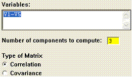
The analysis is again repeated but now extracting only 3 factors (because the scree plot sugested that this was the appropriate dimensionality for these data).
Principal Component Analysis: V1, V2, V3, V4, V5
Eigenanalysis of the Correlation Matrix
Eigenvalue    2.4480    1.6518    0.5110    0.3044    0.0848
Proportion     0.490     0.330     0.102     0.061     0.017
Cumulative     0.490     0.820     0.922     0.983     1.000
Variable         PC1       PC2       PC3
V1            -0.513     0.262     0.479
V2            -0.605    -0.132    -0.229
V3            -0.587    -0.077    -0.383
V4            -0.123    -0.651     0.666
V5             0.101    -0.695    -0.357
Note how all five eigen values are given but only 3 sets of coefficients - for the three retained components - are shown. The interpretation remains the same. PC1 is V1, V2 & V3 while PC2 is mainly V4 & V5. PC3 is relatively unimportant (only 10% of explained variation) and is made up mainly by V1 & V4.