Factor Analysis
Menu Options
This section highlights the main elements in a Factor Analysis using Minitab.
Factor Analysis is accessed from the multivariate menu of the Stats menu.

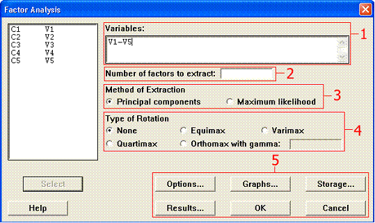
The main factor analysis window has many options, that I have split into
5 sections for explanatory purposes.

Section 1
Obviously you must select some variables to analyse.
Section 2
You should only enter a value here after an initial analysis has suggested
the likely 'dimensionality' of the data. This will always be a number between
1 and the number of variables.
Section 3
Leave this alone! It will always be Principal Components
Section 4
This will either be None or Varimax if you want a rotated solution.
Section 5
There are a variety of additional options accessible via these buttons. These
are described below.
Options:
Don't change any of these.
Graphs:
This is the same as the PCA with the addition of any extra graphs. See the
later analysis for an example.
Storage:
There are 7 options, although the 7th may be 'greyed out'. Only
the first 3 are likely to be of value, although, with the exception of the
scores, they store information that is already presented in the output.
- Loadings: Enter column numbers (one column for each factor) to store the
factor loadings. The rotated factor loadings are stored if you specified
a rotation.
- Coefficients: Enter column numbers (one column for each factor) to store
the factor score coefficients.
- Scores: Enter column numbers (one column for each factor) to store the
factor scores.
- Rotation matrix: this is a matrix used during the rotation - it is of
no interest to you.
- Residual Matrix: this is another matrix that you are unlikely to gain
anything from.
- Eigenvalues: Enter a column to store the eigenvalues.
- Eigenvector matrix: Enter a matrix to store the eigenvectors of the matrix.
Again these are unlikely to be of much value to you.
Results
There are two useful options here. The first sorts the loadings so that the
biggest loadings come first. The second 'blanks' (actually sets them to 0.000)
loadings less than a specified value. 0.2 is a common value used. Remember
these are correlation coefficients so small values could be interpreted as
not being significantly different from 0. The advantage is that it clarifies
which variables are associated with a Factor. An example is given later.
Analyses
Analysis 1
Default options for the PCA_EG1 data file
Factor Analysis: V1, V2, V3, V4, V5
Principal Component Factor Analysis of the Correlation Matrix
Unrotated Factor Loadings and Communalities
  Variable  Factor1 Factor2 Factor3 Factor4 Factor5 Communality
  V1       -0.803*  0.337*  0.342*  0.347* -0.061   1.000
  V2       -0.947* -0.170  -0.164  -0.009   0.219   1.000
  V3       -0.919* -0.099  -0.274  -0.198  -0.178   1.000
  V4       -0.192  -0.837*  0.476* -0.189  -0.005   1.000
  V5        0.159  -0.894* -0.255   0.331  -0.040   1.000
  Variance  2.4480  1.6518  0.5110  0.3044  0.0848  5.0000
  % Var     0.490   0.330   0.102   0.061   0.017   1.000
Factor Score Coefficients
  Variable  Factor1  Factor2 Factor3 Factor4  Factor5
  V1       -0.328    0.204   0.670    1.139  -0.716
  V2       -0.387   -0.103  -0.321   -0.028   2.578
  V3       -0.375   -0.060  -0.536   -0.650  -2.100
  V4       -0.078   -0.507   0.932   -0.619  -0.059
  V5        0.065   -0.541  -0.500    1.087  -0.473
Factor Loadings
What are they and how do they relate to the eigen
vectors?
-
As with the PCA eigen vectors they provide
information about the contribution that each variable makes to a factor.
The most important variables, for each factor, are highlighted by an asterisk
(added by me, not part of the usual output). Note that the pattern is
very similar to those observed in the Minitab PCA of the same data.
-
The factor loadings are obtained from the
eigen vectors by a process of "normalisation" that involves
multiplying each eigen vector by the square root (the singular value)
of its eigen value. For example, for v1 component 1, the PCA eigen vector
is -0.513, and the square root of 2.449 is 1.565: -0.513 x 1.565 = -0.803.
-
If a "pure" PCA is required the
eigen vectors can be obtained from the loadings by dividing each loading
by the square root of the eigen value. For example, -0.803 / 1.565 = -0.513.
- Most usefully the loadings are simple correlation coefficients between
the original variables and the newly derived factors. The matrix plot below
shows these patterns. Examine the salmon pink plots (row 5), which show
the relationships between v1 - v5 and the scores on the first factor. Note
how v1, v2 and v3 are highly correlated. Similarly, examine the pale blue
plots (row 6), v1 - v5 and the factor two scores. This time it is v4 andv5
that are correlated. Thus, we are picking out the same patterns that were
shown by the loadings.

It is also worth noting from the above scatter
matrix that the scores from the five factors (yellow plots in the bottom right)
are uncorrelated (orthogonal) with each other. This property is exploited later
in the multiple regression and discriminant
analysis modules.
Communalities
The first table also gives information about quantities called communalites.
This appears to be rather pointless as all of the entries are 1.000. The communality
concept arises from the fundamental philosophical, and computational, difference
between PCA and FA. This next short section is very important.
Whereas PCA is a variance orientated technique
Factor Analysis is concerned solely with correlations between variables. Factor
Analysis assumes that observed correlations are caused by some underlying
pattern in the data resulting from the presence of a number of predetermined
factors. Strictly, we should know in advance, on the basis of some theory,
how many factors there should be. The contribution of any variable can then
be split into a common component, i.e. that part which contributes to the
factors, and a unique component ('noise'). The sum of the common components
is called the communality. The subsequent FA methodology is very similar to
PCA except that the variability to be partitioned between the factors is that
held in common, unique variability is excluded from the analysis. This makes
sense since we are investigating factors composed of a number of variables,
any unique variance cannot be contributing to a factor, so should be excluded.
Forcing the analysis to use as many factors as
there are variables partially overcomes this difference between PCA and FA.
This is demonstrated by the fact that the communalities are all 1.000, thus
all of the variability is assumed to be common and all of it will be used
in the analysis (as in a PCA).
Factor score coefficients
Factor score coefficients are used to calculate factor scores on the new
factors. For example, the scores on factor 1 are -0.329*V1+-0.386*V2+-0.375*V3+-0.077*V4+0.065*V5
(Assuming that V1 to V5 have first been standardised).
Analysis 2
As above but with sorted loadings and factor scores less than 0.2 blanked
(using options available from the Results button). The only difference between
this and analysis 1 is in the presentation of the information from the analysis.

Factor Analysis: V1, V2, V3, V4, V5
Principal Component Factor Analysis of the Correlation Matrix
Unrotated Factor Loadings and Communalities
Variable  Factor1  Factor2   Factor3   Factor4   Factor5  Communality
V1        -0.803   0.337     0.342     0.347    -0.061    1.000
V2        -0.947  -0.170    -0.164    -0.009     0.219    1.000
V3        -0.919  -0.099    -0.274    -0.198    -0.178    1.000
V4        -0.192  -0.837     0.476    -0.189    -0.005    1.000
V5         0.159  -0.894    -0.255     0.331    -0.040    1.000
Variance   2.4480  1.6518    0.5110    0.3044    0.0848   5.0000
% Var      0.490   0.330     0.102     0.061     0.017    1.000
Sorted Unrotated Factor Loadings and Communalities
These are the same loadings as the previous table but note how the loadings
have been sorted and small loadings set to 0. It is now clear the Factor 1
is variables V2, V3 and V1 while Factor 2 is mainly V4 and V5 plus some V1,
etc.
Variable Factor1  Factor2  Factor3  Factor4  Factor5 Communality
V2      -0.947    0.000    0.000    0.000    0.219    1.000
V3      -0.919    0.000   -0.274    0.000    0.000    1.000
V1      -0.803    0.337    0.342    0.347    0.000    1.000
V5       0.000   -0.894   -0.255    0.331    0.000    1.000
V4       0.000   -0.837    0.476    0.000    0.000    1.000
Variance 2.4480   1.6518   0.5110   0.3044   0.0848   5.0000
% Var    0.490    0.330    0.102    0.061    0.017    1.000
Factor Score Coefficients
Variable Factor1  Factor2  Factor3  Factor4  Factor5
V1      -0.328    0.204    0.670    1.139    -0.716
V2      -0.387   -0.103   -0.321   -0.028     2.578
V3      -0.375   -0.060   -0.536   -0.650    -2.100
V4      -0.078   -0.507    0.932   -0.619    -0.059
V5       0.065   -0.541   -0.500    1.087    -0.473


