MMU - Clustering and Classification

Golden Eagle Core Areas: User pruning of predictors

We are allowed to use some judgement in the selection of predictors. Indeed we should be encouraged to do so since it means that we are thinking more deeply about the problem. Huberty (1994) suggests that we should use three variable screening techniques:

Logical screening:

Uses theoretical, reliability and practical grounds to screen variables. Do some initial research to find variables that may have some theoretical link with our groupings. You may also wish to take into account the data reliability. Finally do not ignore the practical problems of obtaining data, this includes cost (time or financial) factors.

Statistical screening:

Uses statistical tests to identify variables whose values differ significantly between groups. Huberty suggests applying a relaxed criterion, in that we only reject those variables that are most likely to be 'noise' (e.g. F <1.0 or t < 1.0). In addition, examine the inter-predictor correlations to find those variables that are 'highly correlated'. Redundant variables should be removed.

Dimension reduction:

Use a method such as PCA to reduce the predictor dimensionality. This has the additional advantage of removing any predictor collinearity.

This analysis concentrates on statistical screening and applies rather stricter criteria than Huberty suggests. This is because of the need to drastically prune the number of variables. The first step is to carry out a single factor analysis of varaince to find out which variables discriminate between the regions. The F statistics are used to rank the potential predictors. Non-significant predictors (POST< PRE and CAL) have p values <0.05. Note that if a Bonferroni correction for multiple testing is applied the p value of 0.05 for PRE becomes insignificant.

ANOVA
		SS	df	MS	F	Sig.
POST	Between Groups	26.569	2	13.284	2.022	.147
	Within Groups	243.059	37	6.569
	Total	269.628	39
PRE	Between Groups	40.811	2	20.406	3.251	.050
	Within Groups	232.213	37	6.276
	Total	273.024	39
BOG	Between Groups	386.218	2	193.109	18.360	.000
	Within Groups	389.152	37	10.518
	Total	775.370	39
CALL	Between Groups	24.370	2	12.185	2.845	.071
	Within Groups	158.466	37	4.283
	Total	182.836	39
WET	Between Groups	393.277	2	196.638	40.687	.000
	Within Groups	178.819	37	4.833
	Total	572.096	39
STEEP	Between Groups	461.580	2	230.790	21.367	.000
	Within Groups	399.651	37	10.801
	Total	861.231	39
LT200	Between Groups	1265.152	2	632.576	28.273	.000
	Within Groups	827.832	37	22.374
	Total	2092.984	39
L4_600	Between Groups	139.423	2	69.711	8.078	.001
	Within Groups	319.296	37	8.630
	Total	458.719	39

The rank order (based on F statistics) is:

Wet (40.687);
LT200 (28.273);
Steep (21.367);
Bog (18.360);
L4_600 (8.078).

The next analysis is restricted to these 5 predictors.

Do they convey independent information, or are some of them too correlated?

Correlations
		WET	LT200	STEEP	BOG
LT200	Pearson Correlation	-.203	1.000
LT200	Sig. (2-tailed)	.209	.
STEEP	Pearson Correlation	.690	-.547	1.000
STEEP	Sig. (2-tailed)	.000	.000	.
BOG	Pearson Correlation	-.543	-.314	-.462	1.000
BOG	Sig. (2-tailed)	.000	.049	.003	.
L4_600	Pearson Correlation	.266	-.700	.592	-.058
	Sig. (2-tailed)	.097	.000	.000	.722

It is apparent from this table that LT200 & L4_600 are highly correlated (r = -0.700). Since LT200 has the larger F statistic we will exclude L4_600.

Similarly WET & STEEP are highly correlated (r = 0.690). For similar reasons STEEP is excluded.

This leaves WET, LT200 & BOG.

BOG is reasonably correlated with the other two (-0.543 with BOG and -0.314 with LT200), while WET and LT200 have an insignificant correlation (r = -0.203, p = 0.209).

Therefore, exclude BOG and retain only WET and LT200. Now there are the desired 2 predictors (to fulfil the desired cases:predictors ratio). These are now used in a discriminant analysis. (Note that these two predictors were the most important in the previous two analyses.)

top

Summary of Canonical Discriminant Functions

As in the previous analyses we extract two discriminant functions.

Eigenvalues
Function	Eigenvalue	% of Variance	Cumulative %	Canonical Correlation
1	2.930	68.3	68.3	0.863
2	1.359	31.7	100.0	0.759

Wilks' Lambda
Test of Function(s)	Wilks' Lambda	Chi-square	df	Sig.
1 through 2	.108	81.286	4	.000
2	.424	31.327	1	.000

Standardized Canonical Discriminant Function Coefficients
	Function
	1	2
WET	1.033	-0.359
LT200	0.746	0.800

Structure Matrix
	Function
	1	2
WET	0.731	-0.682
LT200	0.328	0.945

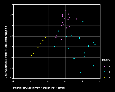
The structure matrix suggests that the first function is primarly associated with wet heath (WET). Cases with a high positive score have more wet heath. The second function comprises both WET & LT200. Larger positive scores are associated with land that has less wet heath and more land below 200m.

As in the other analyses function 1 separates regions 1 and 2, while function 2 separates region 3 from the rest.

Functions at Group Centroids
	Function
REGION	1	2
1	-3.220	-1.058
2	1.495	-0.922
3	-0.081	1.303

top

Classification Statistics

Prior probabilities are set to equal (0.333 for each region).

Classification Results
			Predicted Group Membership			Total
	REGION	1	2	3		Total
Original	Count	1	7	0	0	7
		2	1	12	3	16
		3	0	0	17	17
	%	1	100.0	.0	.0	100.0
		2	6.3	75.0	18.8	100.0
		3	.0	.0	100.0	100.0
Cross-validated	Count	1	7	0	0	7
		2	1	12	3	16
		3	0	0	17	17
	%	1	100.0	.0	.0	100.0
		2	6.3	75.0	18.8	100.0
		3	.0	.0	100.0	100.0

This analysis, based on only two predictors, produces a better discrimination than the one using all 8. It is only marginally worse than the stepwise analysis with 3 predictors (Cross-validated results: region 2 has 1 newly misclassified as region 1 and 1 extra region 3 misclassification).

Scatter of dis2_1 dis1_1 by region

Back to DA examples

Back to Discriminant Analysis

Clustering and Classification methods for Biologists

Discriminant Analysis