MMU - Clustering and Classification

Duchenne Muscular Dystrophy: Discriminant Analysis

All Variables used

The following output was obtained using SPSS.

Class Statistics
Duchenne Muscular Dystrophy		Mean	SD	n
NonCarrier	creatine kinase	43.051	22.206	39
	hemopexin	79.615	12.046	39
	lactate dehydrogenase	12.536	4.788	39
	pyruvate kinase	164.974	39.846	39
Carrier	creatine kinase	155.618	159.854	34
	hemopexin	94.009	11.220	34
	lactate dehydrogenase	26.271	20.665	34
	pyruvate kinase	247.500	67.762	34
Total	creatine kinase	95.479	123.162	73
	hemopexin	86.319	13.658	73
	lactate dehydrogenase	18.933	15.982	73
	pyruvate kinase	203.411	68.269	73

Comparing class means

Which predictors can the two classes be separated on?

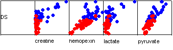
In fact, using an F-test (ANOVA), they differ with repect to all 4 variables. The F statistics are a guide to the extent (reliability) of the differences between the classes for each variable. Using the F values as guide, make a note of the rank order of the predictor variables.

Tests of Equality of Group Means (1 & 71 df)class
	Wilks' Lambda	F
creatine kinase	0.789	18.96
hemopexin	0.720	27.63
lactate dehydrogenase	0.814	16.26
pyruvate kinase	0.631	41.46

Wilk's lambda is a multivariate test statistic whose value ranges between 0 and 1. Values close to 0 indicate that the class means are different and values close to 1 indicating the class means are not different (equal to 1 indicates all means are the same).

top

Correlations and covariances

The following table is presented for information only. It is not normally shown in an SPSS analysis. However, the correlation matrix is useful because it allows us to examine the discriminating variables for evidence of collinearity (correlation - which implies a certain redundancy in the discriminating variables). This can cause problems similar to those observed in multiple regression.

Pooled Within-Groups Matrices(a)
		creatine kinase	hemopexin	lactate dehydrogenase	pyruvate kinase
Covariance	creatine kinase	12140.760
	hemopexin	-35.807	136.176
	lactate dehydrogenase	1244.181	-2.795	210.761
	pyruvate kinase	2273.458	46.802	393.112	2983.936
Correlation	creatine kinase	1.000
	hemopexin	-0.028	1.000
	lactate dehydrogenase	0.778	-0.017	1.000
	pyruvate kinase	0.378	0.073	0.496	1.000

Hemopexin does not appear to be correlated with the other 3 variables, which appear to be related, especially creatine and lactate dehydrogenase. Remember these correlation patterns, they will be relevant later.

Again the next tables are presented for information. An assumption of discriminant analysis is that there is no evidence of a difference between the covariance matrices of the two classs. There are formal significance tests (e.g. Box's M) but they are not very robust. In particular they are generally thought to be too powerful, i.e the null hypothesis is rejected even when there are minor differences, Box's M is also susceptible to deviations from multivariate normality (another assumprion). If Box's test is applied to these data we would conclude that the covariance matrices were not equal. This is not too surprising given the differences, e.g. 493.1 cf 25553.2 and 7.927 & 2667.746.

Covariance Matrices(a)
Duchenne Muscular Dystrophy		creatine kinase	hemopexin	lactate dehydrogenase	pyruvate kinase
NonCarrier	creatine kinase	493.103
	hemopexin	-44.172	145.110
	lactate dehydrogenase	7.927	9.222	22.921
	pyruvate kinase	-6.683	141.737	70.898	1587.710
Carrier	creatine kinase	25553.213
	hemopexin	-26.175	125.889
	lactate dehydrogenase	2667.746	-16.633	427.061
	pyruvate kinase	4899.076	-62.517	764.145	4591.712
Total	creatine kinase	15168.864
	hemopexin	373.443	186.551
	lactate dehydrogenase	1616.947	47.117	255.424
	pyruvate kinase	4585.495	345.821	673.606	4660.662

top

Summary of Canonical Discriminant Functions

Eigenvalues
Function	Eigenvalue	% of Variance	Cumulative %	Canonical Correlation
1	0.994(a)	100.0	100.0	0.706
a First 1 canonical discriminant functions were used in the analysis.

The canonical correlation is the square root of the ratio of the between-groups sum of squares to the total sum of squares. Squared, it is the proportion of the total variability explained by differences between classs. Thus, if all of the variability in the variables was a consequence of the class differences the canonical correlation would be 1, while if none of the variability was due to class differences the canonical correlation would be 0.

Wilks' Lambda
Test of Function(s)	Wilks' Lambda	Chi-square	df	Sig.
1	0.502	47.617	4	0.000

Recall that Wilk's lambda measures differences between classs. It can be converted into a Chi-square statistic so that a significance test can be applied. The null hypothesis to be tested is that 'There is no discriminating power remaining in the variables'. Since p is less than 0.001 we would normally reject Ho. This implies that the variables have some ability to discriminate between the classs.

Note that if p had been >0.05 we would normally halt the analysis since there would be no evidence that our variables were able to discriminate between the classs.

The next table give the standardised values for the coefficients. In other words they are weights that would be applied to standardised variables in order to calculate the discriminant scores.

Standardized Canonical Discriminant Function Coefficients
	Function
	1
creatine kinase	0.402
hemopexin	0.588
lactate dehydrogenase	-0.141
pyruvate kinase	0.641

The predictors can be ranked using these standardised variables (ignoring the sign). This implies that pyruvate kinase is the 'best' discriminator (because its weight indicates that it contributes the most to the discriminant score) and that lactate dehydrogenase is the worst.

Discriminant Score = 0.402.creatine + 0.588.hemopexin - 0.141.lactate + 0.641.pyruvate

Although the coefficients can be used for interpretitive purposes there are problems when, as in this case, there is correlation between the predictors. The weights reflect the contribution made by a varaible, after accounting for the discrimination achieved using other variables. Consider an extreme example of two perfectly correlated predictors (A and B). If A has already been used to discrimate then B cannot provide any extra discrimination (even though on its own it is just as good as A).

The structure matrix is a better index of class differences.

Structure Matrix
	Function
	1
pyruvate kinase	0.766
hemopexin	0.626
creatine kinase	0.518
lactate dehydrogenase	0.480
Pooled within-groups correlations between discriminating variables and standardized canonical discriminant functions Variables ordered by absolute size of correlation within function.

These function values are simply the correlation coefficients between the discriminant score and the predictor variable scores. Note how the strongest correlation is with the pyruvate value. These correlations are shown graphically below.

Plots of predictors against discriminant score

The problem with standardised coefficients is that it is difficult to apply the function to new data. One solution is to obtain unstandardised coefficients. Note that it is not easy to rank these unstandardised coefficients since their magnitudes are related to the scale of their associated predictor.

Unstandardised Canonical Discriminant Function Coefficients
	Function
	1
creatine kinase	0.004
hemopexin	0.050
lactate dehydrogenase	-0.010
pyruvate kinase	0.012
(Constant)	-6.899

Using these values we can construct a discriminant function that can be used to determine a Discriminant Score using raw variables.

Discriminant Score = -6.899 + 0.004.creatine + 0.050.hemopexin - 0.010.lactate + 0.012.pyruvate

The mean discriminant scores for the two classs are shown below.

classUnstandardized canonical discriminant functions evaluated at group means class
	Function
Duchenne Muscular Dystrophy	1
NonCarrier	-0.918
Carrier	1.053

top

Classification Statistics

How well does our discriminant function perform? Allocation of cases to classs is based on a probability calculation that uses Bayesian methods. Part of this calculation demands a knowledge of the prior probabilities, i.e. the probability that a case will belong to particular class in the absence of any other discriminating information. The default calculation assumes an equal probability for each class. In some circumstances they may be unequal, for example if members of one class are very rare then we might expect that class's prior probability to be lower than other classs.

Prior Probabilities for Groups
	Prior	Cases
Duchenne Muscular Dystrophy	Prior
NonCarrier	0.500	39
Carrier	0.500	34
Total	1.000	73

The following are presented for historical purposes. The original method of discriminating between classs was developed by Fisher. In his approach a separate function is derived for each class.

Fisher's linear discriminant function coefficients
	Duchenne Muscular Dystrophy
	NonCarrier	Carrier
creatine kinase	-0.004	0.003
hemopexin	0.567	0.666
lactate dehydrogenase	-0.004	-0.023
pyruvate kinase	0.050	0.073
(Constant)	-27.243	-40.974

The next table contains a lot of information. Firstly, the table rows can be split into two main components:

Original (resubstitution of original cases into the discriminant function)
Cross-validated (The discriminant function is recalculated using all but the current case - the resultant discriminant function is applied to the missing case and a prediction is made. Because the true and predicted class of each case is known a reasonably 'independent measure of the function's predictive power is obtained).

Next the rows. Some are obvious such as case number and actual class. The final column is the discriminat socre for a case. Consider case 1, which has a score of -0.544. The understandardised discriminant function could be applied to the data from the case.

variable x	coefficient (weight)	value	w.x
creatine	0.004	52.0	0.208
hemopexin	0.050	83.5	4.175
lactate	-0.013	10.9	-0.142
pyruvate	0.012	176.0	2.112
constant	-6.899		-6.899
Sum			-0.546

The remaining rows are split into two sections

Highest group (the group which is the most probable, given the discriminant score).
Second highest group (the group with the next highest probability, given the discriminant score).

There are now three columns to consider:

P(D>d \| G=g)	This is the probability of the discriminant score given the predicted class, you can think of this as a type of z test.
P(G=g \| D=d)	P(G/D) is the probability of the group given the discriminant score, hence it is the probability that a case belongs to the predicted class. If the predicted and actual classs are not the same the case is marked ** (for example case 4). P(G/D) is also given for the second most probable class. Note that the probability cutoff is very strict. If P(carrier) = 0.501 and P(non-carrier) = 0.499 the individual would be classified as a carrier. It is important that you examine the probabilities for misclassifed cases to determine if they are a serious or a marginal misclassification. Misclassified individuals can be useful, if you can find out why they were misclassified it may tell you a lot about the nature of the normal differences between classs. For example, suppose you are discriminating between 'normal' and diseased individuals and some normals are predicted to be diseased. What is special about these individuals (possibly other features not included in the analysis) that has kept them healthy?
Squared Mahalanobis Distance to Centroid	A measure of how much a case's values differ from the average of all cases in the class. For a single variable, it is simply the square of the standardized value of the independent variable (because the mean will be 0 for a standardised varaible). A large Mahalanobis distance identifies a case as having extreme values on one or more of the independent variables. Thus, it measures how far a case is from the 'mean' of its class. Note that as this increases the probability of belonging to a class decreases.

Casewise Statistics
		Actual class	Highest class					Second Highest class			Discriminant Scores
			Predicted class	P(D>d \| G=g)		P(G=g \| D=d)	Squared Mahalanobis Distance to Centroid	class	P(G=g \| D=d)	Squared Mahalanobis Distance to Centroid
	Case No.		Predicted class	p	df	P(G=g \| D=d)	Squared Mahalanobis Distance to Centroid	class	P(G=g \| D=d)	Squared Mahalanobis Distance to Centroid
Original	1	1	1	.709	1	.770	.140	2	.230	2.552	-.544
	2	1	1	.833	1	.822	.044	2	.178	3.100	-.708
	3	1	1	.722	1	.776	.127	2	.224	2.608	-.562
	4	1	2(**)	.900	1	.845	.016	1	.155	3.407	.928
	5	1	1	.546	1	.680	.364	2	.320	1.871	-.315
	6	1	1	.806	1	.919	.061	2	.081	4.916	-1.164
	7	1	2(**)	.355	1	.530	.854	1	.470	1.096	.129
	9	1	1	.902	1	.899	.015	2	.101	4.384	-1.041


	39	1	1	.859	1	.831	.031	2	.169	3.218	-.741
	40	2	2	.245	1	.986	1.354	1	.014	9.826	2.217
	41	2	2	.380	1	.553	.771	1	.447	1.195	.175
	42	2	2	.399	1	.974	.713	1	.026	7.926	1.897
	43	2	2	.481	1	.635	.496	1	.365	1.604	.348
	44	2	1(**)	.465	1	.623	.533	2	.377	1.539	-.188
	45	2	2	.099	1	.994	2.726	1	.006	13.119	2.704
	46	2	2	.715	1	.772	.134	1	.228	2.578	.688
	47	2	2	.445	1	.607	.584	1	.393	1.457	.289
	48	2	2	.746	1	.787	.105	1	.213	2.715	.730
	49	2	2	.863	1	.832	.030	1	.168	3.234	.880
	50	2	1(**)	.528	1	.668	.398	2	.332	1.796	-.287
	70	2	2	.446	1	.608	.582	1	.392	1.460	.290
	71	2	2	.540	1	.959	.375	1	.041	6.675	1.666
	72	2	2	.772	1	.798	.084	1	.202	2.828	.764
Cross- validated(a)	1	1	1	.991	4	.765	.283	2	.235	2.649
	2	1	1	.936	4	.815	.819	2	.185	3.783
	3	1	1	.979	4	.771	.439	2	.229	2.862
	4	1	2(**)	.529	4	.893	3.172	1	.107	7.425
	5	1	1	.948	4	.673	.730	2	.327	2.175
	6	1	1	.999	4	.916	.080	2	.084	4.867
	7	1	2(**)	.719	4	.556	2.089	1	.444	2.537
	8	1	1	.763	4	.555	1.850	2	.445	2.294
	9	1	1	.547	4	.890	3.063	2	.110	7.237

	39	1	1	.833	4	.822	1.463	2	.178	4.519
	40	2	2	.102	4	.986	7.722	1	.014	16.195
	41	2	2	.725	4	.531	2.058	1	.469	2.304
	42	2	2	.255	4	.972	5.332	1	.028	12.419
	43	2	2	.413	4	.592	3.951	1	.408	4.693
	44	2	1(**)	.839	4	.650	1.427	2	.350	2.663
	45	2	2	.000	4	.997	36.218	1	.003	47.815
	46	2	2	.670	4	.753	2.362	1	.247	4.596
	47	2	2	.853	4	.594	1.350	1	.406	2.110
	48	2	2	.877	4	.776	1.209	1	.224	3.697
	49	2	2	.953	4	.826	.688	1	.174	3.802
	50	2	1(**)	.038	4	.815	10.147	2	.185	13.116
	59	2	2	.002	4	.999	16.637	1	.001	30.962

	72	2	2	.693	4	.781	2.235	1	.219	4.781
	73	2	2	.306	4	.792	4.819	1	.208	7.494
For the original data, squared Mahalanobis distance is based on canonical functions. For the cross-validated data, squared Mahalanobis distance is based on observations.
** Misclassified case
a Cross validation is done only for those cases in the analysis. In cross validation, each case is classified by the functions derived from all cases other than that case.

Although the case listing can be useful it becomes less useful as the number of cases increases. Often all that is required is a summary of the performance. In the following confusion matrices results are shown for resubstituted (original) data and the more robust cross-validated results. It is the second of these that indicate how well the function is likely to generalise to new cases. The performance is almost always worse using resubstituted data. More information about this can be found in the accuracy pages.

Classification Results(b,c)
			Predicted class Membership		Total
		Duchenne Muscular Dystrophy	NonCarrier	Carrier	Total
Original	Count	NonCarrier	36	3	39
	Count	Carrier	6	28	34
	%	NonCarrier	92.3	7.7	100.0
	%	Carrier	17.6	82.4	100.0
Cross- validated(a)	Count	NonCarrier	35	4	39
	Count	Carrier	6	28	34
	%	NonCarrier	89.7	10.3	100.0
	%	Carrier	17.6	82.4	100.0
a Cross validation is done only for those cases in the analysis. In cross validation, each case is classified by the functions derived from all cases other than that case.
b 87.7% of original grouped cases correctly classified.
c 86.3% of cross-validated grouped cases correctly classified.

This discriminant function appears to have performed quite well, with about 87% of cases correctly classified. Using the cross-validated data 4 non-carriers (10.3%) were classified as carriers and 6 carriers (17.6%) were classified as carriers. Although this may seem quite good we have to question if this level of inaccuracy, particularly the misclassified carriers, would be acceptable in practice. The accuracy pages deal, in greater depth, with the problem of measuring classification accuracy.

Back to DA examples

Back to Discriminant Analysis

Clustering and Classification methods for Biologists

Discriminant Analysis