
Intended Learning Outcomes
At the end of this section students should be able to complete the following tasks.
- Interpret the output from a binary logistic regression of a data file with continuous and categorical predictors.
- Identify those predictors that have a significant effect on the class of a case.
- Calculate confidence limits for a predictor's coefficient.
- Use diagnostic statistics to identify possible problems with an analysis.
- Assess the value of the analysis from the accuracy and the diagnostic statistics.
Background
Suppose that a logistic regression predicts the presence (1) or absence (0) of some outcome using a set of three binary predictors such as gender (A), smoking (B) and colour blindness (C), where one indicates presence and zero absence of that predictor. The following equation was obtained: log odds = -2.7 + 2.5 A - 3.7 B + 1.8 C. The predictor A coefficient of 2.5 is the estimated change in the logarithm of P(presence)/P(absence) for the outcome, when B and C are held constant.
If A, B & C are present (i.e. have the value 1) the log odds are: log odds = -2.7 + 2.5 - 3.7 + 1.8 = -2.1, giving odds of 0.1225 (e-2.1). The 'risk' (probability of outcome 1) is defined by the odds ratio (odds / (1 + odds)). Odds ratios less than one correspond to decreases in the odds as the predictor increases in value while odds ratios greater than one correspond to increases in the odds. If the odds ratio is approximately one, changes in the predictor do not alter the odds of the event. Note that a coefficient of zero is the same as an odds ratio of one (because e-0 is 1.0), both imply the predictor has no effect of the response. In this example the odds, when all predictors have a value of one are 0.1225 / 1.1225 or 0.1091 (10.91%). If A, B and C are absent (all = zero) the log odds equal the constant (-2.7) and the odds are 0.067 (e-2.7 ). This means that 'risk of' of event 1 is 0.067 / 1.067 or 0.063 (6.3%). Therefore, absence of the three predictors almost halves the chance of the event. However, if predictors A and C are present, while B is absent, the log odds are -2.7 + 2.5 + 1.8 = 1.6, giving odds of 4.953 (e-1.6) and a risk of 4.953/5.953 = 0.832 or 83.2%. It appears that the absence of predictor B vastly increases the probability of event 1.
Preliminaries
The previous data set could have been analysed using discriminant analysis because all of the predictors were continuous. However, it becomes more difficult to use discriminant analysis when predictors are categorical. This analysis uses data collected from 87 people (available as an Excel file or a plain text file). The response variable is whether or not a person smoke cigarettes (66 non-smokers and 21 smokers). The five predictors consist of two categorical (gender and ABO blood type) and three continuous (age (years), body mass index (bmi - kg m-2) and white blood cell count (wbc - x 109 l-1)) variables. Because gender has two values it is coded as a single binary predictor (0 = male, 1 = female). Blood group has four categories that must be coded as three dummy predictors. The coding is arbitrary and is shown below. Blood group AB has an implicit coding of zero for each of the three dummy blood group predictors.
| Frequency | Parameter coding | ||||
|---|---|---|---|---|---|
| abo | O | 21 | 1 | 0 | 0 |
| A | 24 | 0 | 1 | 0 | |
| B | 22 | 0 | 0 | 1 | |
| AB | 20 | 0 | 0 | 0 | |
| sex | F | 41 | 1 | ||
| M | 46 | 0 | |||
Null Model
The null model does not include any of the predictors. Instead the only term in the model
is the intercept, whose initial value is:
loge (P(smoke)/P(non-smoke))
= loge 0.241/0.759
= loge 0.318
= -1.145.
| B | S.E. | Wald | df | Sig. | Exp(B) | |
|---|---|---|---|---|---|---|
| Constant | -1.145 | .251 | 20.891 | 1 | .000 | 0.318 |
Model significance
The deviance for the null model is 96.164, which reduces to 75.8 when all of the predictors are added. The reduction in the deviance (20.371) is significant (p=0.005) suggesting that the predictors significantly reduce the unexplained variation. This is further supported by the pseudo-R2 values, although values around 0.3 indicate that a large amount of variation remains unexplained by these predictors.
| Chi-square | df | Sig. | |
|---|---|---|---|
| Model | 20.371 | 7 | 0.005 |
| Step | -2 Log likelihood | Cox & Snell R Square | Nagelkerke R Square |
|---|---|---|---|
| 1 | 75.793 | 0.209 | 0.312 |
Goodness of fit
The Hosmer and Lemeshow test compares observed and expected frequencies in 10 classes. If the model is a good fit the p value, as below, will be greater than 0.05.
| Step | Chi-square | df | Sig. |
|---|---|---|---|
| 1 | 9.004 | 8 | 0.342 |
| smoke = N | smoke = Y | Total | ||||
|---|---|---|---|---|---|---|
| Observed | Expected | Observed | Expected | |||
| Step 1 | ||||||
| 1 | 9 | 8.752 | 0 | 0.248 | 9 | |
| 2 | 8 | 8.429 | 1 | 0.571 | 9 | |
| 3 | 8 | 8.243 | 1 | 0.757 | 9 | |
| 4 | 9 | 8.043 | 0 | 0.957 | 9 | |
| 5 | 6 | 7.647 | 3 | 1.353 | 9 | |
| 6 | 6 | 6.958 | 3 | 2.042 | 9 | |
| 7 | 7 | 6.571 | 2 | 2.429 | 9 | |
| 8 | 7 | 5.722 | 2 | 3.278 | 9 | |
| 9 | 6 | 4.174 | 3 | 4.826 | 9 | |
| 10 | 0 | 1.461 | 6 | 4.539 | 6 | |
Classification accuracy
text block
| Predicted class | Percentage Correct | ||||
|---|---|---|---|---|---|
| non-smoker | smoker | ||||
| Step 1 | Observed class | non-smoker | 62 | 4 | 93.9 |
| smoker | 12 | 9 | 42.9 | ||
| Overall Percentage | 81.6 | ||||
| a The cut value is .500 | |||||
These classification results suggest that this model tends to predict non-smokers quite accurately (93.9% accuracy). However, the accuracy with smokers is poor (42.9%). This inequality between the class predictions is at least partly related to the large difference in the proportions of smokers and non-smokers. If the class allocation threshold is adjusted (from 0.50 to 0.28) to match the class proportions in the sample data the overall accuracy declines to 73.6% but the number of smokers correctly predicted rises from 9/21 to 14/21. The decline in overall accuracy is a consequence of more false identifications of non-smokers as smokers. Possible solutions to the problems created by unequal class proportions are covered by the accuracy page.
Model structure
text block
| B | S.E. | Wald | df | Sig. | Exp(B) | 95% LCL | 95% LCL | ||
|---|---|---|---|---|---|---|---|---|---|
| Step 1(a) | bmi | -0.214 | 0.096 | 4.942 | 1 | 0.026 | 0.807 | 0.669 | 0.975 |
| age | 0.031 | 0.038 | 0.682 | 1 | 0.409 | 1.032 | 0.958 | 1.110 | |
| wbc | 0.632 | 0.214 | 8.705 | 1 | 0.003 | 1.882 | 1.236 | 2.864 | |
| sex(1) | -0.188 | 0.615 | 0.094 | 1 | 0.760 | 0.829 | 0.248 | 2.764 | |
| abo | 3.685 | 3 | 0.298 | ||||||
| abo(1) | -1.290 | 0.885 | 2.124 | 1 | 0.145 | 0.275 | 0.049 | 1.560 | |
| abo(2) | -0.430 | 0.762 | 0.319 | 1 | 0.572 | 0.651 | 0.146 | 2.895 | |
| abo(3) | -1.335 | 0.814 | 2.688 | 1 | 0.101 | 0.263 | 0.053 | 1.298 | |
| Constant | -0.034 | 2.775 | 0.000 | 1 | 0.990 | 0.967 |
It is not surprising that age and blood group are not good predictors (p>0.05) of smoking habits (see above). It is less obvious if gender should be a significanr predictor. In these data gender does not predict smoking (p=.760). Only bmi and wbc are significant predictors. The probability of smoking appears to decline as bmi increases (negative coefficient). Because bmi is a measure of obesity (weight corrected for height) this suggests if two people are the same height, but different weights, the lighter person is the most likely to smoke. The coefficient for wbc is positive, suggesting that the probability that a person smokes is greater if their white blood cell count is larger. There is a well known relationship for white blood cell counts to be higher in smokers.
ROC analysis
The earlier classification table suggested that the model had an overall accuracy of 81.6%. The calculator from the accuracy page estimates that Kappa (0.422) is only just above the 0.4 threshold that is usually taken to indicate poor agreement.
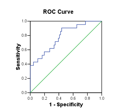
There are two main problems with these accuracy assessments. Firstly, they are based on the training data and are likely to be over-optimistic (see the accuracy page). Secondly, they assume that the 0.5 cut-point is appropriate. It is generally better to assess accuracy with a threshold-independent measure from a ROC plot. The ROC plot below has an AUC of 0.895 (std error = 0.057), with 95% confidence limits of 0.671 and 0.895. These figures suggest that the model is reasonably accurate.
Diagnostics
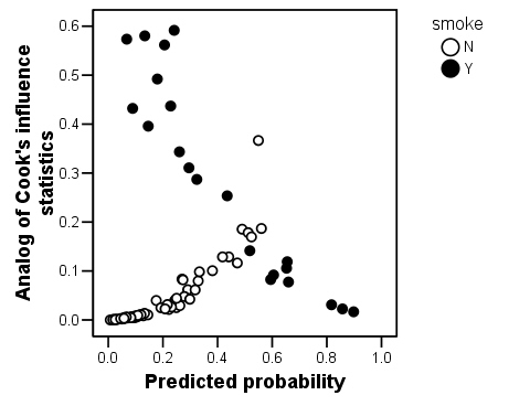
Cook's Distance (D) measures the influence of an observation by estimating how much the other residuals would change if the case was removed. Its value is a function of the case's leverage and of the magnitude of its standardized residual. Normally, D > 1.0 identifies cases that might be influential. An arbitrary threshold criterion of D > 1.0 is normally used to identify influential cases. None of the cases in this analysis have a D value < 1, suggesting that none of the case is creating problems.